Timestamp Embeddings

A continuous temporal geometry for transformers, proven in two domains, with a larger purpose.

The Claim

Every transformer ever trained has a representation of where in a sequence a token sits. Positional embeddings encode this (Vaswani et al., 2017). The geometry of meaning inside the model is shaped by two things: what each token is, and where it sits relative to its neighbors. This works. It is the basis of every language model that has ever been built, and it makes the model fluent at any task that maps onto reasoning over ordered character streams.

But the world the model is asked to reason about is not a sequence of slots. It is a continuous timeline with periodic structure at every scale, all active at once. Days, weeks, seasons, years, decades, all simultaneously present in any timestamp. The same date carries information at every scale. A transformer with no geometric axis for this structure can still reason about it, but it has to do so through the same relational machinery it uses for everything else. The result is what frontier models actually demonstrate today: brittle, notation-dependent, approximate temporal reasoning that breaks under reformulation and fails on anything that depends on duration or interpolation rather than recall of named moments.

This paper specifies a timestamp encoding that adds the missing axis. It takes a raw scalar (seconds since epoch) and produces a learned vector representation in which periodic structure at every scale is a first-class geometric property. The encoding has been proven in two distinct domains. Its mechanism is general. The architecture is in service of a larger argument about what becomes computable once time enters the latent space as a primitive rather than a shadow.

Two embeddings, two different questions. Position is about order inside a single read. Timestamp is about location inside history. The model needs both.

What Positional Embeddings Cannot Do

It is worth saying directly what is being added, by saying what is missing.

A transformer’s latent space is a relational manifold. Word embeddings encode co-occurrence statistics. Attention computes relevance between embeddings. The geometry of the resulting space is a map of meaning-relations learned from text. This is powerful for sequential reasoning over discrete tokens. It is also static, with no dedicated continuous axis for time. The meaning of a word, the relevance between two tokens, the geometry of a concept cluster, these are fixed properties of the trained model. Context modulates activation patterns. The underlying space does not move.

What temporal capability exists in frontier models is brute-forced through this same relational machinery, and there is exactly one path by which it gets there. Somewhere in the corpus a human wrote down a temporal relationship in prose. After that, X happened. X caused Y. Here is our company’s timeline. In the weeks following the announcement, A then B then C. Whenever a writer has already done the work of relating events to each other in text, the model absorbs that relation through ordinary next-token prediction over the prose that carries it. That is the only way time enters the model.

It is not enough that the events were recorded with timestamps. They have to be recorded with timestamps in a passage of text that also relates them to each other. If a hundred different forums describe whistleblower events separately, each post anchored to its own moment, and no piece of text anywhere in the corpus ever ties them together into an ordered account, the model has no way to form a representation of how they sequence. The information is on the substrate. There is no architectural mechanism that lifts it into a representation. Disparate timestamp tokens scattered across the corpus do not stitch into a continuous timeline. The model can only learn what some writer has already worked out for it.

The resolution that sits inside the corpus is enormous. Trillions of social-media posts carry second-precision timestamps. News articles carry datelines. Logs, broadcast transcripts, court records, scientific publications, and journals are paired with explicit time markers at every scale, from microseconds in event logs to minutes in posts to hours in articles to days in editorials to years in retrospectives. None of that resolution becomes a high-resolution representation of any domain’s actual sequence of events. The moments live in different files, different documents, and unless someone has written a piece of bridging prose that ties them into an ordered account, they never meet in text that explains how they relate. A trillion parameters, expended to fluently read whatever sequence a writer has already laid out while leaving cross-document timelines structurally out of reach, is evidence the architecture does not have the structure the task wants.

And even with that scale, the failure is observable as soon as the task requires anything other than recall of named moments. Ask a frontier model how long a task will take and the answer drifts across phrasings, varies with notation, and breaks under reformulation. Ask how much time has passed since an event and the answer is unreliable. Ask about a date adjacent to one well-covered by training and the model cannot interpolate; it can only retrieve. This is not a calibration problem. It is the absence of a continuous geometric axis to compute against.

Prior work has attempted to retrofit temporal awareness onto language models without changing the structure of the latent space. Rosin and Radinsky (2022) extend transformer self-attention to condition on the timestamp metadata associated with training texts, producing time-aware contextualized word representations and improving semantic-change detection across historical periods. Farhan et al. (2023) propose a diffusion-based temporal word embedding model that captures how the contexts of words and entities shift over time in a timestamped corpus. Both approaches improve recall of time-anchored language but inherit the same structural issue: the temporal information lives as additional relational structure layered over a static manifold rather than as a dedicated geometric dimension. With enough data they sharpen the surface proxy. Neither produces a continuous timeline.

This was tested directly in the development of this work. Long before any timestamp encoding was written, the question was: can a frontier model be taught a personal timeline by fine-tuning alone, by manufacturing the bridging prose the architecture is structurally dependent on? A stream of timestamped first-person thoughts was processed into hierarchical summaries (daily, then weekly, then monthly). Each summary was the exact kind of writing the architecture absorbs natively: a passage in which the temporal relations between events are stated in prose. The summaries were then used as fine-tuning data with prompts of the form “what did this person think about on [date].” Thousands of prompt-completion pairs. Dates rendered in many formats. Hierarchical summaries giving the model multiple paths to any given moment. The full apparatus that would, if synthesized bridging text were enough, let a model build a timeline by being explicitly fine-tuned on one.

The recall did not hold up. Even on dates the model had explicit training data for, the answer often was not what happened on that date. The model leaned into semantic association instead. Concepts that were related to each other got reported as having been conceived the same day, even when they were actually conceived years apart. The semantic neighborhood overrode the temporal one because the semantic neighborhood is where the architecture actually lives. Phrasing variations did not patch this. The fine-tuning data deliberately included many ways of asking about the same date, and the model still could not generalize to any linear timeline at small scale. Ask about a date adjacent to a trained one and the model cannot interpolate. Ask about elapsed time between two events and the answer is unreliable. The dates became surface anchors. They did not become coordinates. Without a continuous geometric axis for time, “the day after” cannot be computed. The model can only retrieve, not interpolate, and even the retrieval lands wherever the latent space’s semantic neighborhood pulls it rather than at the date the question asked for.

Pipe a raw Unix timestamp into the same model and the relational proxy has even less to hold onto. The number 1766966400 is tokenized into subword chunks, embedded into the same semantic space as every other token, and processed through the same relational attention. Whatever weak temporal associations a frontier model brute-forced from surface text are largely stripped out at this notation. The architecture has no native mechanism for extracting periodicity from a scalar or for computing temporal distance between two scalars; whatever temporal reasoning it does manage still comes back through the same relational machinery, statistically rather than geometrically. The temporal axis remains a shadow, not a coordinate.

The same model fed the string “December 25, 2025” activates Christmas associations, gift-giving, winter. Not because it understands the date as a point on a continuous timeline, but because those tokens co-occur in training data with those concepts. The Christmas association is statistical proxy. It is brittle. It vanishes the moment you change notation. The two representations encode the same moment in time. The model does not know this.

This is not a calibration problem. It is not solved by scale. The geometry of the latent space is constrained by the operations that produce it. Embedding lookup, linear projection, dot-product attention. These operations define a relational manifold. No amount of data or parameters adds a temporal axis to that manifold, because the operations themselves have no mechanism for continuous periodic structure. Scaling improves the surface proxy. It does not produce time.

The failure modes that follow are structural. A model with no temporal axis cannot reliably tell you how long a task will take, because duration is not representable in a space with no continuous axis for it. It cannot distinguish a claim that is early from a claim that is wrong, because both register as out-of-distribution and the only available measure is symmetric distance from the centroid. It cannot track the momentum of a discourse, the trajectory of a belief, the recurrence of a cycle, because none of these are properties of any individual snapshot. They are properties of motion across snapshots. The model has access only to the snapshot.

What the Encoding Does

Take a single scalar, seconds since epoch. Send it through two parallel pathways, one for aperiodic trend, one for periodic rhythm. Blend them with an adaptive gate that learns per domain how much of each pathway the task needs. The output is a learned vector in which the geometric relationships between any two timestamps reflect the actual temporal relationship between them, at every scale at once.

The trend pathway is a small MLP that captures direction. Time accumulates. Things drift, grow, decay. The pathway is initialized tiny, regularized with heavy dropout, and scaled down before reaching the gate, so that the model starts by relying on periodic structure and only recruits trend if the loss demands it. This prevents the trend pathway from memorizing the training set as a near-linear function of time, which is the failure mode it would otherwise default to.

The periodic pathway is a bank of sinusoidal oscillators. Earlier work on learnable representations of time established that a learned mapping from a raw scalar timestamp can outperform fixed positional encodings on time-series tasks. Time2Vec (Kazemi et al., 2019) defines a model-agnostic vector representation that combines one linear component with a bank of periodic components, each with its own learnable frequency and phase. Xu et al. (2019) construct translation-invariant time kernels grounded in Bochner’s theorem, producing explicit functional feature maps for time intervals between events. T-Rep (Fraikin et al., 2024) jointly learns a feature extractor and a set of time embeddings as part of a self-supervised representation-learning objective for time series. The pathway here extends this line of work in two ways: by replacing the single periodic bank with a multi-band initialization that covers many orders of magnitude, and by training the periodic pathway jointly with a regularized trend pathway under an adaptive gate, rather than concatenating it with an unregularized linear component.

Each oscillator has a learnable frequency, stored in log-space, and a learnable phase. The frequencies are initialized across four logarithmic bands covering thirteen orders of magnitude, from sub-second to multi-decade. The multi-scale receptive-field intuition behind this initialization mirrors the dilated-convolution approach to spanning long-range dependencies across scales (Yu and Koltun, 2016). The training strategy is selection rather than design. Initialize oscillators at every conceivable time scale, then let gradient descent prune and sharpen the ones that match the data’s actual periodicities. Because frequencies live in log-space, a small parameter update can shift an oscillator smoothly from a daily cycle to a weekly one. The model discovers which scales matter rather than being told.

The two pathways are blended by a learned gate. Two details matter. First, the gate sees the combined representation with its gradient detached, so that the gate cannot kill a pathway by driving its routing weight to zero through gradient flow. Both pathways must become useful on their own terms. The gate only learns to route, not to shape. Second, the first layer of the gate has spectral normalization applied, which bounds its Lipschitz constant and keeps routing weights stable. The model can rebalance smoothly between trend and periodic. It cannot mode-switch sharply or extinguish one pathway entirely.

The result, after training, is a vector representation in which the geometric relationship between two timestamps is the actual temporal relationship between them. Two moments twenty-four hours apart have a specific geometric relationship in this space regardless of how they are formatted, because the encoding has discovered a daily frequency band and aligned its oscillators to it. Two moments a year apart have a different but equally precise relationship. The temporal dimension is not a relational shadow. It is a geometric primitive.

The Normalization Insight

This is the piece that took the longest to find and is what makes the encoding deployable.

The base encoding operates on raw seconds. In practice this creates two problems for the trend pathway. The input is order one billion, which a single linear layer struggles to project stably, and the dynamic range across datasets varies by many orders of magnitude. Normalizing the input to the unit interval solves both problems for the trend path.

But naive normalization breaks the periodic path. The periodic pathway computes the sine of (input times frequency). The gradient with respect to a frequency parameter is (input times cosine), and the magnitude of that gradient scales linearly with the input. When the input is raw seconds, the frequency parameters receive a strong training signal and the oscillator bank learns. When the input is normalized to the unit interval, the gradient is roughly one billion times smaller. Frequency learning effectively stops. The periodic pathway dies. The model can no longer discover periodicities in the data.

The trend path wants a normalized input. The periodic path needs a large input to keep frequency learning alive. These are not the same input. The encoding sends different inputs to the two pathways. The trend path receives the normalized scalar. The periodic path receives the normalized scalar scaled back up by the dataset’s actual time range, recovering the gradient magnitude that frequency selection requires. The dataset bounds are stored as fixed buffers. The gating, the detach, the spectral norm, all of it is preserved.

This is the standard form of the encoding. It is what trains stably on any time range, from microseconds to centuries, without sacrificing the gradient signal that drives the geometry.

Definition

The complete standard form, consolidated. The encoding maps a scalar timestamp τ to a vector e(τ) ∈ R^d.

Inputs and buffers. A scalar timestamp τ (seconds since epoch). Two non-trainable buffers per dataset, τ_min and τ_max, with range Δτ = τ_max − τ_min.

Trainable parameters at output dimension d:

Trend MLP: W₁ ∈ R^(d×1), W₂ ∈ R^(d×d) (and biases). W₁ initialized uniform on [−1e-5, +1e-5].
Periodic bank: log-frequencies f ∈ R^d initialized with d/4 entries each from the four bands [−20, −10], [−10, 0], [0, 6], [6, 12]. Global frequency scale α ∈ R, initialized to 1. Phase offsets φ ∈ R^d, initialized N(0, 1).
Gate MLP: W_g^(1) ∈ R^(4d×2d) (spectral-normalized first layer), W_g^(2) ∈ R^(2×4d).
LayerNorm parameters for the trend branch and the periodic branch.

Forward pass.

Normalize once:

τ_norm = (τ − τ_min) / (Δτ + ε)

Trend branch (operates on the normalized input):

u = LayerNorm( W₂ · GELU( Dropout_0.5( W₁ · τ_norm ) ) ) * 0.1

Periodic branch (rescales the normalized input back up by Δτ to preserve the gradient on f):

τ_scaled = τ_norm · Δτ
freqs    = exp(f) · α
v        = LayerNorm( sin( τ_scaled · freqs + φ ) )

Gate (input detached so gradients do not flow back into u or v):

g = softmax( W_g^(2) · GELU( W_g^(1) · stop_grad([u ; v]) ) )    g ∈ Δ¹

Output:

e(τ) = g[0] · u + g[1] · v ∈ R^d

Details that matter. The 0.1 factor on the trend branch and the tiny initialization on W₁ together suppress the trend pathway early in training so the encoding starts by relying on periodic structure. The gate’s stop_grad prevents the gate from killing a pathway through gradient flow; the spectral norm on W_g^(1) keeps routing smooth. The asymmetric input (τ_norm for trend, τ_scaled for periodic) is what lets the encoding train stably on any dataset’s time range without collapsing the gradient on the frequency parameters. Removing any one of these breaks the encoding in a way the next sections describe.

What the Context Window Becomes

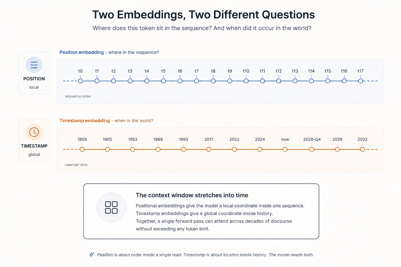
A positional context window is a ruler with fixed markings. N slots, uniform spacing, fixed resolution. Slot one before slot two before slot three. You cannot subdivide a slot. You cannot put something between position two and position three. Resolution and range are locked together. If you want to see more of the timeline, you need more slots. If you want finer granularity within a fixed slot count, you cannot have it.

A timestamp context window is a different kind of object. It is a set of N containers placeable anywhere on a continuous timeline. The same number of containers can span fifty years or a hundred milliseconds. The range is decoupled from the container count. The resolution comes from the frequency bands, not the slot count. The density can be non-uniform. You can cluster most of your context around one critical month and scatter the rest across a decade, and the model attends across that irregular distribution because the temporal structure is in the encoding, not the index. The containers are unordered. Shuffling them changes nothing. Each container says only “here is an observation, and here is when it happened.”

The context window becomes continuously subdivisible. Given a hundred containers, you can place them across five decades or across a hundred milliseconds and the same architecture handles both, because the multi-band initialization covers all scales and gradient descent selects the relevant ones. The grid becomes a field. The ruler becomes a timeline.

This is not an incremental improvement on positional encoding. It is a different kind of representational object, one in which temporal trajectory is computable as geometry rather than approximated through co-occurrence.

Domain One: Time-Series Forecasting

The encoding has been tested as a component of a forecasting transformer. Each context point carries a value and a timestamp. Values are embedded through a linear projection. Timestamps are encoded through the gated dual-pathway module. The two are concatenated, and the resulting context is processed through self-attention layers. A target future timestamp is then encoded through the same module, paired with a zero in place of the unknown value, and used as the query for cross-attention over the processed context. The future timestamp asks the context what its value should be.

This is the core architectural pattern. The timestamp encoding gives the query rich temporal structure, and the attention mechanism finds the context points most relevant to that temporal position. A data point from one Tuesday can attend to data points from previous Tuesdays if the encoding has learned a weekly frequency. A data point from one summer can attend to data points from previous summers if the encoding has learned an annual one. The temporal structure is in the geometry, not the position index.

The critical test is the random-context regime. Twenty-five points are sampled from earlier in the sequence, predicting a random future point. The model cannot rely on recency or ordering. It must use the actual timestamps to understand temporal relationships. Without timestamp encoding, the model has twenty-five values at unknown times and must predict a value at an unknown time. With encoding, it has twenty-five (value, time) pairs and a target time, a much richer signal.

The encoding consistently outperforms the no-encoding baseline. The gap is larger on the random regime than on the ordered regime, because that is where temporal reasoning is essential. The same architecture works across time scales spanning seconds, days, or years, because the multi-band initialization covers all scales and gradient descent selects whichever periodicities the data actually contains.

The model also learns when to rely on trend and when to rely on cycles. On data with strong periodicity, the gate routes toward the periodic pathway. On data with directional drift, it routes toward trend. On data with both, it blends. The allocation is adaptive and learned per domain.

Domain Two: Trust Over Time

The same encoding is used in a trust-attention transformer, with a different surrounding architecture and a different task. The shift is from “what value at this time” to “which source can I trust at this time.”

Multiple sources make predictions. Each source’s expertise follows a sinusoidal cycle, and at any moment exactly one source is the expert. The expert outputs the true value. The non-experts output noise. The model receives the source predictions and a timestamp and must output the expert’s value. Success means the model has learned not to average the predictions but to select the right one based on who is reliable when.

The token structure has four equal-width slots. A projection of the value. The timestamp encoding. A source embedding (a learned vector per source, updated as the model trains). And the elementwise product of the timestamp encoding and the source embedding. This last slot is doing real work.

The reason is algebraic. When source expertise follows a sinusoid in (time plus source-phase), the angle-addition identity decomposes that expression into a bilinear combination of a time term and a source term. The product space directly represents (this source, at this time), which is what trust attention needs to learn. Concatenation requires the downstream MLP to learn the cross-terms implicitly. Elementwise multiplication encodes the cross-terms by construction. The token structure now matches the structure of the trust signal.

Each training sample carries multiple timestamps, placed evenly within a single span. The span size is drawn log-uniformly from a minimum window up to the full date range. Different samples see different spans, so the model encounters the expert cycle at every scale within individual training examples. Loss is computed across all targets per sample, producing a much denser gradient signal than a single-timestamp regime.

Self-attention runs across all the time-source pairs in the sample. The model can attend across time, across sources, and across (time, source) pairs simultaneously. Cross-attention then uses the timestamp encoding itself as the query: each target timestamp asks the context “which source should I read out at this moment.” The same architectural pattern as the forecasting transformer, with a richer context and a different readout.

The ablation discipline is strict and the result is sharp. The model exposes flags that remove the temporal pathway, the source pathway, or both. When the temporal pathway is removed, the timestamp encoding is dropped and cross-attention is replaced with mean pooling, so that no time information can leak through the query. When the source pathway is removed, the source embedding is dropped. Across both task configurations, the three reduced ablations (value-only, value plus time, value plus source) all score at chance. Only the full model (value, time, source, and the multiplicative interaction) learns. Source, time, and content are all required. Any two of the three collapses to chance.

This is the trust triplet. It is not a tuning result. It is a structural property of the mechanism. The proof translates: best test accuracy of 88.5% on the harder configuration (eight sources, chance 12.5%), and 96.7% on the easier configuration (three sources, chance 33.3%). The encoding’s gate routes the harder configuration strongly toward periodic, because source expertise is purely cyclical and the trend path has nothing to add. The gate suppresses what is not needed.

Why the Same Encoding Works in Both Domains

The two architectures look different. One asks “what value at this time,” the other asks “which source at this time.” The surrounding token structure differs. The number of attention heads, the depth, the dataset, all differ. But the encoding is identical in form, and its role in the architecture is identical.

In both cases the encoding gives a query rich temporal structure so that attention can find the context most relevant to when the model is being asked about. In the forecasting case, the target timestamp asks the context what its value should be. In the trust case, the target timestamp asks the context which source to read out. The mechanism is the same. What changes is what the context contains and what is being read out from it.

This is the property that makes the encoding general. It is not a trick tied to a specific architecture. It is a temporal-geometric primitive that slots into any attention mechanism that needs to reason about when. The gating, the multi-band initialization, the normalization, the detach, all of these are domain-agnostic. They produce a vector representation of time that has the geometric structure time actually has. Any task in any modality that depends on temporal structure can use it without modification.

The Generalization

The mechanism is not specific to numerical data. It is a property of attention itself once the embedding spaces include source and time. Wherever a transformer is attending to anything, the same triplet can be made readable.

In language models that mediate between human sources, journalists, experts, witnesses are sources. Their claims are content. When they made the claims is time. A journalist who consistently breaks accurate stories in a domain earns higher attention weight in that domain. A source whose predictions age well gains influence. The attention distribution over sources at a given time is the trust score, not a secondary computation, the mechanism itself.

In image generation, the artists in the training distribution are sources. The pixels are content. When the work was made is time. An image that strongly references one painter’s style should show concentrated attention on that painter’s work, with a long tail across related sources, and a residual contribution attributable to the artist directing the model. The provenance is the attention distribution. The receipt is the mechanism.

In music generation, the musicians whose tracks shaped the training distribution are sources. The waveforms or spectrograms are content. The same triplet, the same gated combination, the same attention. The chord progression that does not resolve where expected, the timbre that sits between categories, the rhythmic feel that is not quantized to any standard grid, these are contributions the model cannot source from any single training track. They show up as residual. The musician’s work is readable as the gap between what the model would have produced and what it produced under direction.

In code generation, the repositories are sources. The tokens are content. A function that closely mirrors a specific implementation has concentrated attention on that source. A function assembled from patterns across hundreds of repositories has diffuse attention. The licensing implications are readable directly from the weights.

In scientific instruments, multiple sensors measuring the same phenomenon are sources. Each measurement is content. A sensor that drifts in cold weather gets low attention weights in winter and high weights in summer. This is the same computation as a forecaster who is accurate during elections but unreliable between them. The data type changes. The mechanism does not.

In every case, the same triplet: source, time, content. The same gates. The same softmax. The same interpretable attention distribution. The mechanism is the receipt.

The timestamp encoding is the piece that makes the time dimension first-class in all of these. Without it, the source and content embeddings can still combine through standard attention, but the model has no native representation of when. It is left with relational proxies whose handling of 1766966400 and “December 25, 2025” is largely incommensurate even though both encode the same moment in the world. With the encoding, the temporal dimension becomes a continuous, periodic, scale-invariant geometric structure that the rest of the attention mechanism can compose with.

What This Makes Possible

The largest claim is not architectural. It is epistemic.

A system that filters on consensus at a single time slice is structurally incapable of detecting novelty. Distance from the centroid is a scalar. It tells you how far a claim is from the center of the current distribution. It says nothing about whether the center is moving toward that claim or away from it. To distinguish novelty from noise, you need a vector. You need to know the direction the distribution has been moving. A claim that is out of distribution today but lies along the trajectory of belief motion over the past several years is geometrically different from a claim that is equally far out but orthogonal to that trajectory. The first is a candidate for early signal. The second is a candidate for noise. They are indistinguishable without the temporal axis.

This is the reason every system trained on current consensus suppresses the voices that prove most valuable in hindsight. Semmelweis on hand washing. Patterson on lead contamination. Carson on pesticides. Stewart on radiation. Each looked far from the center of consensus at the time. Each lay along the trajectory the distribution was about to take. The institutions evaluating them had only the scalar measure. By that measure, they looked wrong. They were early.

A model with timestamp embeddings does not solve this by being more open-minded. It solves it by giving the latent space a geometry that can represent which way the distribution has been moving. A claim, a source, a concept now carries a temporal coordinate. The same semantic content at different temporal coordinates occupies different points in the latent space. The space is no longer a manifold. It is a field. And in a field, trajectories are computable.

The Prophet Incentive becomes mechanical in this geometry. A source whose stakes were peripheral to consensus at time T, but whose predictions the field later moved toward, accrues attention weight in similar future contexts. The track record is not a tally. It is the sampling weight the attention distribution reveals when the model is later asked about the domain. The credit is in the geometry.

Social Proof of Impact becomes mechanical in the same geometry. A source whose staked actions were followed by community discourse encoding the desired outcome materialized accrues weight on the action side. The temporal axis carries both. Past prediction accuracy and past consequential action both show up as motion in the field, and the attention distribution updates accordingly.

The trust triplet that the trust transformer demonstrates is the structural minimum required for any of this to work. Content alone gives the static manifold. Content plus source tells you who, but not when they were reliable. Content plus time tells you what was said when, but not whose track record to weight it against. Only the full triplet enables the geometry in which novelty and impact are distinguishable from noise and accident.

What Doesn’t Work

It is worth being precise about what the encoding replaces.

Fixed-frequency positional encodings (Vaswani et al., 2017) assume evenly spaced positions and predetermined scales. They cannot adapt to the data’s actual periodicities and do not handle irregular timestamps. They were designed for token positions in a sequence, not moments on a continuous timeline.

Learned time representations from the prior literature, of which Time2Vec (Kazemi et al., 2019) is the canonical example, combine one linear component with a learnable periodic bank without regularization, gating, or multi-band initialization. Kernel-based functional time representations (Xu et al., 2019) embed time intervals through translation-invariant kernels and explicit feature maps but do not introduce a separate trend pathway or an adaptive gate. Time-series representation methods that jointly learn time embeddings with a feature extractor (Fraikin et al., 2024) advance the use of time embeddings for self-supervised pretext tasks but inherit the same single-pathway structure. On the random-context forecasting regime, encodings of this kind learn more slowly and generalize worse, because they lack the inductive bias that the multi-band initialization and the gate provide.

Retrofitted temporal attention over standard language-model latent spaces (Rosin and Radinsky, 2022; Farhan et al., 2023) improves time-anchored recall but, as discussed above, treats time as additional relational structure layered on top of a static manifold rather than as a dedicated geometric axis. The encoding here moves the temporal information into the geometry itself.

Calendar decomposition (embed hour, weekday, month, year separately and concatenate) works when those are the right features. It fails when the relevant periodicity is, say, eleven days, or three and a half cycles across an arbitrary range. It also cannot handle sub-day timestamps or multi-year trends without manual extension. It puts the human in the loop for feature selection, which is exactly the work the encoding is designed to remove.

Naive normalization (scaling timestamps to the unit interval before feeding to both pathways) breaks frequency learning by collapsing the periodic gradient signal. The asymmetric normalization described above is the fix.

Removing the gate detach lets the model learn a degenerate solution in which the gate kills one pathway by driving its weight to zero through gradient flow. The detach forces both pathways to become useful independently. Without it, the model can collapse onto the trend pathway and overfit by memorizing the training set’s timestamp-to-value mapping.

These are not opinions. Each was confirmed by ablation against the architecture described above. Each represents a degree of freedom that has been pinned by the requirements of stable training and faithful temporal geometry.

Closing

The encoding takes a single number and produces a vector in which the geometric relationships between any two timestamps reflect the actual temporal relationships between them, at every scale at once. It does this through learnable oscillators spanning thirteen orders of magnitude, blended with a regularized trend pathway through an adaptive gate, with an asymmetric input transformation that lets it train stably on any time range. It has been proven in two distinct domains: time-series forecasting, where the target timestamp queries a context window of past observations, and trust learning, where the target timestamp queries a context of source predictions and reads out which source to trust. The mechanism is identical in form across both. The same encoding works because the encoding is doing the same thing in both: giving a query rich temporal structure so that attention can find the context most relevant to when.

The encoding generalizes because it is not specific to any domain. It is a temporal-geometric primitive that slots into any attention mechanism over any modality. Wherever a transformer attends to anything that exists in time, the same three embedding spaces (source, time, content) can be made first-class, the same gates can compose them, and the resulting attention distribution can be read as provenance. The mechanism is the receipt.

The larger purpose is epistemic. A static manifold cannot distinguish a claim that is early from a claim that is wrong, because the only measure available is symmetric distance from the centroid. A time-varying field can, because trajectory is computable in it. The encoding is what lifts the manifold into a field. Once that lift is made, novelty becomes detectable, track record becomes geometry, and the truth no longer has to win today. It has to outlast the noise. And a system whose latent space can represent the momentum of beliefs across time will learn, from the structure of the field itself, which signals are moving toward the center of truth and which are decaying away from it.

This is the architecture that makes that possible.

References

Vaswani, A., Shazeer, N., Parmar, N., Uszkoreit, J., Jones, L., Gomez, A. N., Kaiser, Ł., and Polosukhin, I. “Attention Is All You Need.” NeurIPS, 2017.
Kazemi, S. M., Goel, R., Eghbali, S., Ramanan, J., Sahota, J., Thakur, S., Wu, S., Smyth, C., Poupart, P., and Brubaker, M. “Time2Vec: Learning a Vector Representation of Time.” 2019. arXiv:1907.05321.
Xu, D., Ruan, C., Korpeoglu, E., Kumar, S., and Achan, K. “Self-Attention with Functional Time Representation Learning.” NeurIPS, 2019.
Fraikin, A., Bennetot, A., and Allassonnière, S. “T-Rep: Representation Learning for Time Series using Time-Embeddings.” 2024. arXiv:2310.04486.
Rosin, G. D., and Radinsky, K. “Temporal Attention for Language Models.” Findings of NAACL, 2022.
Farhan, A., Barranco, R. C., Akbar, M., and Hossain, M. S. “Temporal Word Embedding with Predictive Capability.” Knowledge and Information Systems 65(12), 2023.
Yu, F., and Koltun, V. “Multi-Scale Context Aggregation by Dilated Convolutions.” ICLR, 2016.
Ash, J. “Iris and Ŧrust: A Technical Framework for Democratic Belief Coordination.” Cognicism, 2024.
Ash, J. “Novelty, Noise, and Time.” Cognicism, 2026.
Ash, J. “Ŧrust Across Dimensions: Provenance as Attention Over Source, Time, and Content.” Cognicism, 2026.
Ash, J. “Why Positional Embeddings Are Still Valuable.” Cognicism, 2026.
Ash, J. “The Dimensionality Gap: Why Transformers Can’t Tell Time.” Cognicism, 2026.
Ash, J. “The Context Window: Positional Embeddings vs Timestamp Embeddings.” Cognicism, 2026.