Source Embeddings

Same object as a word embedding. Different index. Different question.

Abstract

A source embedding is a fixed-length vector of learnable parameters assigned to a single contributor in a corpus, optimized through gradient descent against a downstream objective. Structurally it is identical to a word embedding: the same dimensionality, the same random initialization, the same lookup operation at inference, the same gradient updates during training. The only difference is what the embedding indexes. Word embeddings have one row per word in the vocabulary. Source embeddings have one row per speaker in the population. Every contribution that source ever makes looks up the same row, which is what turns the vector into a stable representation of the contributor’s identity rather than a description of any single piece of content they produced.

The construction is not new. Amir et al. (2016), Li et al. (2016), and Yang and Eisenstein (2017) all train per-speaker vectors of word-embedding dimensionality through standard end-to-end backpropagation, and the geometry of the resulting source matrices clusters speakers by behavioral similarity in the same way word matrices cluster tokens by semantic similarity. The mechanism is also empirically sufficient for reliable source identification: the trust attention proof discussed below demonstrates that a per-source embedding, when combined with a timestamp encoding and their multiplicative interaction, allows a transformer to select the correct source at a moment in time it has never seen, while every reduced configuration collapses to chance.

The downstream consequence is that authorship and trust become first-class properties of the architecture. Attention distributions over source embeddings serve as direct, decomposable receipts of which contributors influenced which outputs and how much. The same mechanism that made meaning into geometry through word embeddings can make authorship into geometry through source embeddings. The mechanism has been in the literature for a decade. What remains is to use it.

The Claim

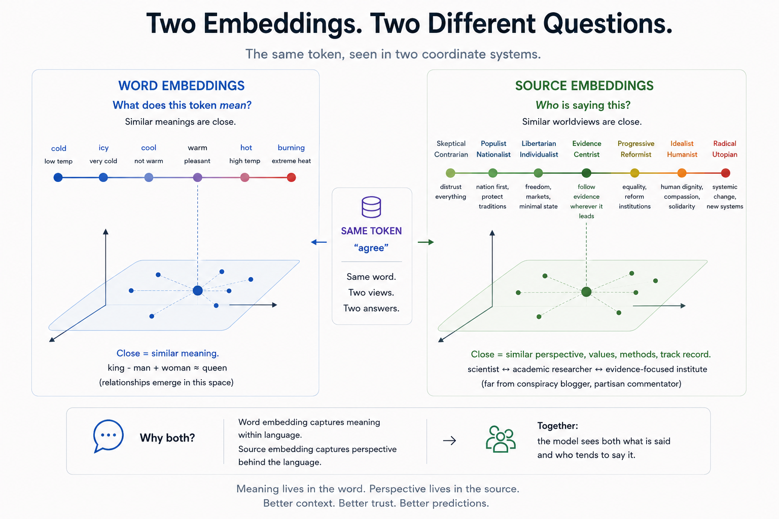
A source embedding is the same kind of object as a word embedding. Same dimensionality, same random initialization, same gradient updates, same lookup at inference. The difference is the index. A word embedding matrix has one row per word in the vocabulary. A source embedding matrix has one row per speaker, author, account, or sensor in the population of contributors to the corpus. Word embeddings answer the question of what a token means. Source embeddings answer the question of who is saying it.

This is not novel. Amir et al. (2016) trained word and user matrices side by side for sarcasm detection, with the two matrices sharing dimensionality d and feeding into the same classifier. Li et al. (2016) gave each speaker in a conversational model a “K dimensional speaker-level representation,” where K is exactly the word embedding dimensionality, and stated explicitly that these “speaker embeddings are learned jointly with word embeddings and all other parameters of the neural model via backpropagation.” Yang and Eisenstein (2017) carried the construction further by giving each author a vector pretrained from their position in a social network and using it to attend over basis classifiers.

The architecture has been sitting there for a decade. What is missing is not the mechanism. What is missing is the deployment.

What a Word Embedding Is

It is worth pausing on the canonical case, because the parallel to source embeddings is exact and the parallel only carries weight if the canonical case is described correctly.

A word embedding is a row of a matrix. Pick a vocabulary, fix a dimensionality, instantiate a matrix with one row per word and d columns, initialize the entries to small random values. That matrix is the embedding. Every time the network processes the word at vocabulary index i, it looks up row i and uses the resulting d-dimensional vector as input to whatever comes next. The lookup is a hard assignment. The vector is the entirety of what the model knows about that word at the input layer.

Training updates these rows through gradient descent. If the objective is next-word prediction, the gradient flows back through whatever attention or recurrence layers sit between the embedding and the loss, and it lands on the row corresponding to the word that was looked up. The row moves. Across millions of examples, the rows for words that co-occur with similar neighbors are pushed in similar directions, and the rows for words that co-occur with different neighbors are pushed apart. The geometry of the resulting matrix is the geometry of co-occurrence statistics in the training corpus.

This is what Mikolov et al. (2013b) observed when they reported that vector arithmetic in the trained embedding space produces results like vec(Madrid) minus vec(Spain) plus vec(France) approximately equals vec(Paris), or the more famous king minus man plus woman approximately equals queen. The geometry of the space encodes semantic relationships, because the operations that produced the geometry were sensitive to the contexts in which words appeared together. Nothing about the structure forces this. It is a property that emerges from the training objective applied to enough data.

Pennington et al. (2014) gave the same structure a more direct construction. Their objective fits vector representations to global word-word co-occurrence statistics through weighted least squares, with the dot product of two word vectors trained to equal the log of how often those words co-occur. The result is a different training procedure for the same kind of object: an embedding matrix in which the rows encode meaning through geometry. Different recipe. Same product.

The thing to hold onto is that none of this required anything special about words. The procedure works on any discrete entity for which a meaningful context can be defined. Words and their neighbors are the simplest case. Speakers and the contributions attributed to them are another. The structure is general.

Same Object, Different Index

Source embeddings index a population of speakers in the same way word embeddings index a vocabulary. Pick a population, fix a dimensionality (the same d as the word embeddings, by construction), instantiate a matrix with one row per speaker, initialize the entries to small random values. Every time the model processes content attributable to source j, it looks up row j and uses the resulting d-dimensional vector as part of the input. The lookup is a hard assignment. The vector is the entirety of what the model knows about that source at the input layer.

Training updates these rows the same way. The gradient that flows back to a source vector reflects how much that source’s identity helped or hurt the loss on a given example. Across many examples, sources that contribute in similar ways are pushed in similar directions. Sources whose contributions diverge are pushed apart. The geometry of the resulting matrix encodes a notion of similarity between speakers, derived from their actual contributions, in exactly the same way that the geometry of a word embedding matrix encodes a notion of similarity between words.

Amir et al. (2016) stated this construction directly. They define a user embedding matrix U with one column per user, each column a d-dimensional vector, and note that the parameters of this matrix can be initialized randomly. Their word embedding matrix E has the same form: one column per word, each column a d-dimensional vector. The two matrices live in the same space, concatenate into the same classifier, train against the same loss. After training, a t-SNE projection of U separates users by political alignment and sports interest, demonstrating that the resulting geometry is doing the same work for users that the geometry of E does for words. Different population. Same object.

Li et al. (2016) constructed the same parallel for conversational dialogue. Each token in their model “denotes a word token that is associated with a K dimensional distinct word embedding.” Each speaker in their model has a “K dimensional speaker-level representation.” Same K. Same training. They observe explicitly that the resulting speaker space behaves like a relational manifold: “two speakers who sound distinctly British, and who are therefore close in the vector space” allow the model to generalize from training data on one speaker to predictions about the other. The geometric analogy of king minus man plus woman approximately equals queen has its persona-space counterpart in this generalization, though Li et al. do not state it as vector arithmetic.

Yang and Eisenstein (2017) extended the construction by deriving the author vectors from a social network rather than from the text itself. Each author was embedded according to their position in the Twitter follower graph, then those vectors were used to compute attention weights over a small bank of sentiment classifiers. The same author vector that locates a speaker in social space turns out to locate them in linguistic space, because of linguistic homophily. Same object. Trained against a different signal. The downstream use is the same.

What the source embedding captures is whatever the training signal can express about the source. If the signal is next-word prediction in the source’s own posts, the embedding learns to encode that source’s lexical style. If the signal is sentiment classification across many authors, the embedding learns to encode the source’s typical sentiment patterns. If the signal is downstream prediction accuracy where the source is one of many forecasters contributing to a consensus, the embedding learns to encode the source’s reliability as a forecaster. The geometry of the source matrix encodes whatever the gradient asked it to encode. Nothing more, nothing less.

What the Source Embedding Encodes

Word embeddings, after training, place semantically similar words near each other. “Cold” sits near “icy” and “cool.” “Warm” sits near “pleasant” and “mild.” The temperature dimension emerges from the training data, because words used in similar contexts develop similar embeddings.

Source embeddings, after training, place behaviorally similar sources near each other. A skeptical contrarian sits near other skeptical contrarians. A progressive reformist sits near other progressive reformists. The clusters that emerge depend on what aspect of the source the training signal exercises. If the signal exercises the source’s worldview, sources with similar worldviews cluster. If the signal exercises the source’s track record at predicting outcomes, sources with similar accuracy patterns cluster. If the signal exercises both, both kinds of clustering coexist in the same space, on different axes.

A scientist with a long track record of accurate evidence-based reasoning ends up near other evidence-focused contributors, in the same way “cold” ends up near “icy.” A conspiracy blogger with a track record of unreliable predictions ends up far from both. The distance is not asserted in advance. It is learned, the same way semantic distance between words is learned, from the patterns the training data actually contains.

This matters for downstream use. The same retrieval and arithmetic operations that work on word embeddings work on source embeddings, because the underlying object is the same. Cosine similarity between two source vectors is a measure of behavioral similarity. Nearest-neighbor lookups identify sources that contribute in similar ways. The decomposition of an attention distribution over sources tells you which sources contributed to a given output and how much. None of this requires new mechanism. It is the standard interface for an embedding matrix, applied to a different population.

Proof of Identifiability

The trust attention proof described in the timestamp embeddings paper takes this construction and uses it as one of the three required inputs to a reliable source-selection mechanism. The architecture treats each source as a discrete entity, assigns each one a d-dimensional learnable vector, and trains the vectors jointly with the rest of the model against a downstream task: given a set of source predictions at a target timestamp, output the value of the source who is the expert at that time.

The ablation result is the relevant evidence. Four model configurations train on the same task. The baseline has access to content only. The temporal-only model has access to content and time. The source-only model has access to content and source. The full model has access to content, time, source, and the multiplicative interaction of time and source. All four use the same architecture. The only difference is which embedding spaces are active.

All three reduced configurations score at chance. The full model trains to 88.5% on the harder configuration (eight sources, chance 12.5%) and 96.7% on the easier configuration (three sources, chance 33.3%). The interpretation is immediate. Content alone is insufficient. Content plus time is insufficient. Content plus source is insufficient. Only content plus source plus time, with the multiplicative interaction that algebraically corresponds to the structure of the ground truth, lets the model learn who to read out when.

The source embedding’s role in this is to identify. The model needs to distinguish the contribution of source A from the contribution of source B, even when their content is similar, because the rule that determines correctness depends on which source produced which value. The source matrix is the mechanism by which the model performs this identification. Each source’s vector is its label in the model’s latent space, learned from the gradients its contributions generate during training. The proof demonstrates that this label is reliable: once the source matrix and the timestamp encoding are both present, the model can predict which source’s prediction to trust at a future moment it has never seen, because the source’s identity is geometrically distinguishable in the latent space.

This is not a special property of the trust transformer. It is a property of source embeddings as a class of objects. The lookup is hard. The vector is the source’s identity. Once the matrix is trained, the model can refer to any source by its row, and that reference is as reliable as the reference to any word by its row in the word embedding matrix. The mechanism is the standard one. The application is to sources rather than to words.

Two Coordinate Systems

The same utterance can be projected into two embedding spaces. One projection is the word embedding lookup: each token gets its row from the vocabulary matrix, capturing what the token means. The other projection is the source embedding lookup: the speaker gets their row from the source matrix, capturing who they are. The two projections are independent. The two matrices live in the same dimensionality and operate through the same gradient mechanism, but they index different populations and answer different questions.

A model that consumes both projections sees the utterance from both sides. It sees the content, located in the meaning manifold that word embeddings define. It sees the source, located in the perspective manifold that source embeddings define. The downstream attention layers combine these into a single representation that reflects both what was said and who said it. This is not a hypothetical architecture. It is the construction Amir et al. (2016) use, the construction Li et al. (2016) use, the construction Yang and Eisenstein (2017) use, the construction the trust transformer uses.

The framing matters because most language models do not do this. A frontier language model trained on the open internet consumes the utterance through only one projection. The word embedding lookup is performed. The source lookup is not, because there is no source matrix. The training corpus contains text from millions of authors, but their identities have been stripped before training. The model sees only the words. The result is a system that can produce fluent output in any style by interpolating across the styles its training data contained, while remaining structurally unable to attribute that output to any specific contributor or to weight contributions by the track records of their authors.

The two-coordinate-system framing makes the missing axis visible. There is a place in the architecture where authorship belongs. The mechanism for storing it is the same mechanism the model already uses for storing meaning. The decision not to use that mechanism is a decision, not a constraint. It is implemented by training without source tags, not by any architectural limitation of the transformer.

This is the point on which a great deal hangs. If the architecture refuses authorship, every output is a remix of contributions whose origins have been deliberately erased, and the model cannot truthfully say where any given response came from. If the architecture accepts authorship, every output carries an attention distribution over sources, and that distribution is a direct, readable receipt of which contributors influenced what was produced. The two cases use the same underlying machinery. The difference is whether the source matrix is instantiated.

The Box Metaphor

There is a way to describe what this gives back to the people whose words built the model, and the description is not metaphorical. It is the literal behavior of an embedding matrix with one row per speaker.

A word embedding gives every word in the vocabulary the same number of parameters. The word “the” gets a d-dimensional vector. The word “petrichor” gets a d-dimensional vector. Neither word is allocated more space than the other to represent its meaning. The constraint is uniform, by construction.

A source embedding gives every speaker in the population the same number of parameters. A speaker whose corpus contribution is millions of words gets a d-dimensional vector. A speaker whose contribution is a single comment gets a d-dimensional vector. Neither speaker is allocated more space than the other to represent their perspective. The volume of what a speaker has said is captured at training time through the gradient signal. The space they are given to be represented in is uniform.

This is the property that makes source embeddings a candidate primitive for representative aggregation. Every speaker has a box of the same size. The box can be filled with as much nuance as the speaker’s actual contributions support. The construction does not privilege the loud. It does not silence the quiet. It allocates representational space uniformly, then lets gradient descent determine the position of each row based on what each speaker actually contributed. A speaker who has said little ends up near other speakers who said similar things, because that is where the gradient places them. A speaker who has said a lot ends up at a position that reflects the totality of what they said, but not at a position that takes up more of the matrix than anyone else’s.

This is the technical underpinning of what John Ash, in earlier work on Cognicism, has described as a citizen embedding. The construction is identical to the source embeddings already in the literature. The framing changes. Where Amir et al. (2016) used user embeddings to improve sarcasm classification, the same object can be used to give every contributor to a model’s training data a per-speaker representation that the model can attend over, weight by reliability, and decompose into attribution at inference time. The underlying mechanism is the standard one. What is new is the deployment at scale, against a corpus large enough that the population of source embeddings starts to look like a population of citizens.

What This Makes Possible

Once source embeddings are first-class, the architecture has a place to put attribution. Per-source attention distributions become decomposable. Trust scores become geometry, in the same way that semantic relationships in word space became geometry through the work of Mikolov et al. (2013a, 2013b) and Pennington et al. (2014). The mechanism that decides which sources contributed to an output is the same mechanism that decides which tokens to attend to in standard self-attention, applied to a different population.

The trust transformer demonstrates the floor of this. Given a set of source predictions and a target timestamp, the model learns which source to read out based on the source’s reliability at that time. The reliability information is not encoded as metadata; it is encoded in the geometric position of the source’s vector relative to the other source vectors and to the temporal context. The output is not just a value. It is an attention distribution over sources, and that distribution is the trust score.

The same construction lifts to higher content dimensionalities without changing form. In a language model that has been trained with source tags, every generated token carries an attention distribution over the source matrix. The journalist whose work shaped the model’s coverage of a topic appears as a peak in the distribution when that topic is generated. The witness whose claims age well accrues weight in the distribution when similar contexts arise. The contributor whose contributions are noise gradually loses weight. None of this requires a separate trust-scoring system. The attention distribution is the trust score, as a property of the mechanism itself.

In an image model trained with source tags on the artists whose work appears in the corpus, the same decomposition is available. Each generated image carries an attention distribution over the source matrix of artists, and the distribution is a direct receipt of which artists’ work most influenced the output. Provenance becomes a property of the architecture rather than a property of an external audit system. The artist whose style the model is referencing appears as a peak. The artists who contributed broader patterns appear as a long tail. The output is decomposable.

The political consequence is the one that warrants stating directly. A model that erases source identity at training time cannot give it back at inference time. A model that retains source identity at training time can attribute its outputs to specific contributors, weight contributions by reliability, and structurally support an economy in which the people whose work built the model receive accurate credit for that work. The mechanism for this is the source embedding matrix. The mechanism has been in the literature for a decade. The decision not to use it is what produces a model that launders authorship at scale.

Closing

Source embeddings are a known structure. They have a clean prior literature. They are the same kind of object as word embeddings, share the same dimensionality, train through the same gradient mechanism, and produce a relational manifold with the same kind of geometric structure. The trust transformer proof demonstrates that the construction is sufficient to support reliable source identification at training time, generalizing to source-time configurations the model has never seen.

The contribution of this paper is not to introduce the mechanism. The contribution is to articulate the two-coordinate-system framing that makes the architectural symmetry visible: the same utterance is a token in two parallel embedding spaces, one that captures what is being said and one that captures who is saying it. The mechanism is symmetric. The choice to use only one of the two coordinate systems in frontier language models is a deployment decision, not a structural one.

A language model with source embeddings as a first-class input is not a research proposal. It is a model that uses one additional standard component, instantiated against a corpus where source attribution exists. The infrastructure question is whether the corpus retains attribution. The architectural question is whether the model has a row per source. If both answers are yes, the model returns authorship as a property of its own outputs, by the same mechanism that lets it use word vectors to construct meaning.

Word embeddings made meaning into geometry. Source embeddings make authorship into geometry. Together they make every utterance decomposable into what is being said and who is saying it. The system that holds both is a system in which credit and attribution become as computable as fluency. The mechanism is already in place. The remaining work is to use it.

References

1. Bengio, Y., Ducharme, R., Vincent, P., and Jauvin, C. “A Neural Probabilistic Language Model.” Journal of Machine Learning Research 3, 2003, pp. 1137 to 1155.
2. Mikolov, T., Chen, K., Corrado, G., and Dean, J. “Efficient Estimation of Word Representations in Vector Space.” ICLR Workshop, 2013. arXiv:1301.3781.
3. Mikolov, T., Sutskever, I., Chen, K., Corrado, G., and Dean, J. “Distributed Representations of Words and Phrases and their Compositionality.” NeurIPS, 2013. arXiv:1310.4546.
4. Pennington, J., Socher, R., and Manning, C. D. “GloVe: Global Vectors for Word Representation.” EMNLP, 2014, pp. 1532 to 1543.
5. Amir, S., Wallace, B. C., Lyu, H., Carvalho, P., and Silva, M. J. “Modelling Context with User Embeddings for Sarcasm Detection in Social Media.” CoNLL, 2016, pp. 167 to 177.
6. Li, J., Galley, M., Brockett, C., Spithourakis, G. P., Gao, J., and Dolan, B. “A Persona-Based Neural Conversation Model.” ACL, 2016. arXiv:1603.06155.
7. Yang, Y., and Eisenstein, J. “Overcoming Language Variation in Sentiment Analysis with Social Attention.” Transactions of the ACL 5, 2017, pp. 295 to 307.
8. Vaswani, A., Shazeer, N., Parmar, N., Uszkoreit, J., Jones, L., Gomez, A. N., Kaiser, Ł., and Polosukhin, I. “Attention Is All You Need.” NeurIPS, 2017.
9. Ash, J. “Iris and Ŧrust: A Technical Framework for Democratic Belief Coordination.” Cognicism, 2024.
10. Ash, J. “Timestamp Embeddings.” Cognicism, 2026.
11. Ash, J. “Will AI Take Over the Government?” 2023.